Relaxing a Skyrmion
2,304 spins walk downhill and a magnetic whirl appears
Relaxing a skyrmion: minimisation in a magnet
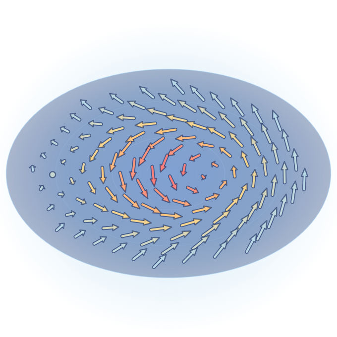
In Part 1 the energy depended on two numbers and in Part 2 on eleven. Here it is the energy of a small magnet: 2,304 spins on a lattice, each free to point in any direction. Start from a rough guess, let the minimisers walk downhill, and a magnetic skyrmion appears: a whirl of spins that cannot be smoothed away, and whose size is set by the twisting interaction between the spins and by the field.
Inspired by the practical session of Philipp Rybakov at the POLYTOPO Training School, Budapest 2025 (acknowledgement).
Standings
Iterations of each method. ✓ at rest (largest torque below 10−8 J), … cut off. A field evaluation is one pass over all spins, the costly part of every step.
Convergence
Skyrmion number
The model and the method
A square lattice of 48 × 48 classical spins of unit length, ni, that repeats periodically in both directions. The energy has three parts:
E = −J Σ ni·nj − Σ Dij·(ni × nj) − B Σ niz
The exchange J makes neighbouring spins parallel. The Dzyaloshinskii–Moriya interaction (DMI) makes them twist: here its strength is D = 0.3 J. The field B points along z, out of the screen.
Units: J is the exchange constant, not the joule. Energies, the torque and the field are all given in units of J. B stands for the energy of one spin in the field: its magnetic moment times the field strength. Energies are counted from the uniform state, in which all spins point along the field.
Every step keeps the spins on the unit sphere: each spin moves along the part of the step direction that is perpendicular to the spin, and is then scaled back to unit length. For the two methods with a line search, the energy along the step is approximated by a parabola and the step goes to its minimum; it is halved if the energy does not fall.
A run stops when the largest torque is below 10−8 J: the spins are then at rest. It is cut off after 200,000 iterations. The fixed step starts at 0.2 and is halved whenever the energy would rise.
A state at rest need not be a minimum: a perfectly symmetric state can stay balanced on a ridge of the energy. To prevent this, every start, and every state after a change of the field or of the twist, is tilted at random by up to about 0.001 radian. A state that comes to rest after that is almost always a minimum. Very close to a field at which a state loses its stability, a walk can still stop on a ridge that is almost flat.
Not included: the long-range magnetic (dipole–dipole) interaction, anisotropy, temperature, and the third dimension. The spins are classical vectors of fixed length. The iterations are not time steps: a minimiser only looks for a state at rest and does not follow the real motion of the spins.
How to use
- Press Relax and watch the three methods bring the spins to rest.
- Change the field B or the twist: the spins relax again from where they are.
- Choose another start, or point at a place and press + Skyrmion here to add one.
- Click a method to see its spins.
Reading the picture
You look at the lattice from above, with the field pointing towards you.
Dark spins point along the field, white spins against it. Colours show the direction of spins that lie in the plane, as on the small wheel in the corner. The arrows show the same in-plane direction.
Numbers: energies, the torque and the field B are given in units of J, the exchange constant between neighbouring spins (not the joule).
From this page to a real magnet
A magnetic skyrmion is a few nanometres to a few hundred nanometres across. A regular lattice of skyrmions was first observed in the chiral magnet MnSi in 2009, by neutron scattering. Skyrmions are studied as possible carriers of information, because they are small, can be stable and are easy to move.
Its skyrmion number is the same integer that counts the coverings of the sphere by the polarisation skyrmions of light: the map from the plane to the sphere is the same, only the arrows are now magnetic moments.
Research codes do what this page does, for millions of spins in three dimensions, and they add the long-range magnetic interaction between all pairs of spins. Computing that interaction efficiently was the second subject of the practical session at the Training School.
The pictures during a relaxation are not a film of the real motion. In a real magnet the spins precess around their fields and lose energy by damping, while a minimiser is free to take any path that leads downhill. Only the state at rest has a physical meaning.
They also have to choose among many minima. Which state a real magnet is found in depends on its history: how the field and the temperature were changed, just as the result here depends on the start.
The formulas behind the picture
Energy: E = −J Σ⟨ij⟩ ni·nj − Σ⟨ij⟩ Dij·(ni × nj) − B Σi niz, with |ni| = 1 and the sums over pairs of nearest neighbours, each pair counted once. With rij the unit vector from spin i to spin j: Bloch Dij = D rij, along the bond; Néel Dij = D rij × z, across it.
Effective field: Hi = −∂E/∂ni = J Σj nj + Σj nj × Dij + B z, an energy, in units of J. Only its part perpendicular to the spin can turn it: gi = Hi − (Hi·ni) ni, of the same size as the torque |ni × Hi|. Here g points downhill; in Part 1, g was the slope, which points uphill. At a minimum every spin is parallel to its field. The reverse does not hold: the torque also vanishes on a ridge or on a peak of the energy.
Step: ni → (ni + α di) / |ni + α di|, with d = g for the two gradient descent methods and d = g + β dold for conjugate gradient (Polak–Ribière–Polyak β, with the old vectors projected onto the new tangent planes).
Skyrmion number: N = (1/4π) ∫ n·(∂xn × ∂yn) dx dy. On the lattice it is the sum of the signed solid angles of the spherical triangles spanned by neighbouring spins, divided by 4π, which is always an integer.
The practical session “Numerical energy minimization in magnetics” by Philipp Rybakov (University of Uppsala, Sweden) at the POLYTOPO Training School on Physics and Mathematics of Topological Textures, Budapest, 12–13 May 2025, on the conjugate gradient method and on ways of keeping the spins on the unit sphere.
This simulation continues Part 1 and Part 2, which are based on the C++ code written by Philipp Rybakov for that session. The spin model on this page and its implementation are not taken from his code.
Yorgis Androulakis, IACM / FORTH
Have a suggestion to improve this simulation?