Polarisation Skyrmions
A beam that covers the whole sphere
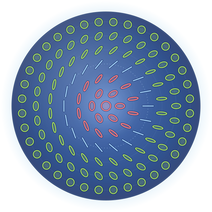
Polarisation skyrmions: a beam that covers the sphere
In Part 1 one beam of light had one polarisation, i.e. one point on the Poincaré sphere, and in Part 2 optical elements moved that point around. Real beams can carry a different polarisation at every point of their cross-section, so the whole beam is a map to the sphere. Some beams cover the sphere completely, once or several times: these are polarisation skyrmions, and the number of coverings is a topological invariant.
The beam on the sphere
Each coloured ring of the beam is drawn here as a loop on the sphere, the grey spokes as lines joining them. The white dot is the probe. Drag to turn the sphere.
Skyrmion number
At the probe
The beam in this simulation
Two Laguerre–Gauss modes with the same width w(z) in the two circular polarisations: a Gaussian u₀ in C₊ and a vortex mode uℓ ∝ r|ℓ| eiℓϕ u₀ of charge ℓ in C₋,
E = u₀ ê₊ + (c eiα uℓ + ε u₀) ê₋
Only the ratio μ = E₋ / E₊ = ε + c (√2 r/w)|ℓ|/√|ℓ|! · ei(ℓϕ + α − |ℓ| arctan(z/zR)) matters for the polarisation. It fixes the point on the sphere: S₃ = (1 − |μ|²)/(1 + |μ|²), S₁ + iS₂ = 2μ/(1 + |μ|²).
For ε = 0 the centre of the beam is C₊ (north pole), and far from the axis the light tends to C₋, which is reached exactly only in the limit r → ∞. This is Part 1's stereographic picture seen from the other pole: for ℓ = 1 the beam's cross-section is the projected plane.
ℓ is the vortex charge of the C₋ mode. For this family of beams the skyrmion number equals ℓ; in general it is not tied to a single mode index.
The beam is paraxial, monochromatic and fully polarised at every point. Both modes have radial index p = 0 and the same waist, so they share the width w(z) and the wavefront curvature and differ only in their Gouy phase. N(R) is summed numerically on a grid of points, so its last digit is approximate.
How to use
- Move the mouse (or drag a finger) over the beam: the probe shows the local polarisation and its point on the sphere.
- ℓ sets how many times the texture winds. R is the part of the beam that is counted.
- c, α, ε deform the texture, and z lets the beam travel.
- Switch the background between S₃, the Skyrme density, the longitude φ and the intensity.
Reading the pictures
Red regions have S₃ > 0, green regions S₃ < 0 (as in Part 1), and dark lines mark linear polarisation.
The Skyrme view shows the skyrmion density ρ = S·(∂ₓS × ∂ᵧS)/4π: how much of the sphere each part of the beam covers, per unit area. Its total over the beam is the skyrmion number N.
Why this is topology
The beam's cross-section is a plane and its polarisation defines a map from that plane to the sphere S². Far from the axis the polarisation tends to a single state, so the plane behaves like a sphere too, and the map has an integer degree: how many times it wraps S² around itself.
That degree is the skyrmion number N = (1/4π)∫ S·(∂ₓS × ∂ᵧS) dx dy. Smooth changes cannot alter an integer, so N survives deformations and free propagation, as long as the field vanishes nowhere and the light far from the axis keeps tending to a single state. It is the same invariant that classifies magnetic skyrmions in thin films, studied in other POLYTOPO working groups.
Optical skyrmions like these have been made in the lab with shaped laser beams, and higher-dimensional versions cover the larger state spaces of non-paraxial light. This was the topic of M. A. Alonso's talk at the Heraklion workshop.
The formulas behind the picture
Ratio of the circular components: μ(x, y) = E₋/E₊ = ε + c (√2 r)|ℓ|/√|ℓ|! · ei(ℓϕ + α − |ℓ| ψG), with r and ϕ the polar coordinates in units of the beam width w(z), and the Gouy phase ψG = arctan(z/zR).
Point on the sphere: S = (2 Re μ, 2 Im μ, 1 − |μ|²) / (1 + |μ|²). Intensity I ∝ e−2r²(1 + |μ|²).
Skyrmion number inside the window: N(R) = (1/4π) ∫r<R S·(∂ₓS × ∂ᵧS) dx dy, which tends to N = ℓ as R → ∞ for this family of beams. Numerically it is summed exactly as the signed solid angle of small spherical triangles.
The talk “Covering spheres and higher order compact manifolds with optical fields” by Prof. Miguel A. Alonso (Institut Fresnel, Centrale Méditerranée & University of Rochester) at the POLYTOPO Workshop on Emerging Applications of Topological Textures, Heraklion, Crete, 16–19 September 2026.
This simulation extends Part 1, which is based on an original Mathematica notebook by Prof. Miguel A. Alonso (Institut Fresnel, Centrale Méditerranée & University of Rochester), presented at the POLYTOPO Heraklion Workshop 2026. See the acknowledgement in Part 1.
Yorgis Androulakis, IACM / FORTH
Have a suggestion to improve this simulation?