The Energy Landscape
Seven ways to walk downhill to the minimum
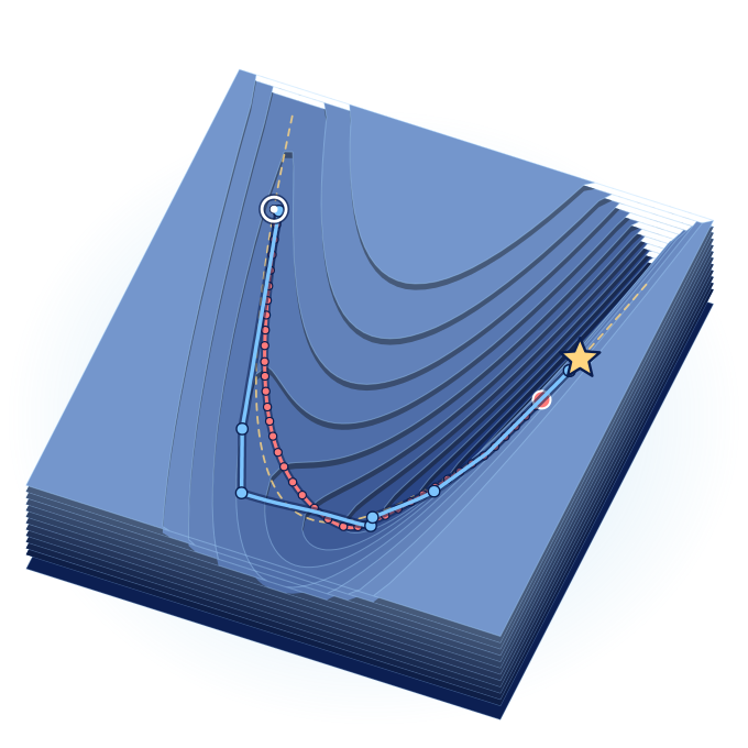
The energy landscape: walking downhill to the minimum
Stable magnetic textures, such as domain walls and skyrmions, are states in which the energy of the magnet has a local minimum: no small change lowers it. To find them on a computer, one starts from a guess and walks downhill on the energy landscape, step by step. Here the energy depends on only two numbers, so the whole walk can be drawn on a map, and seven ways of choosing the next step can be compared, from plain gradient descent to Newton’s method.
Based on the C++ code written by Philipp Rybakov for the POLYTOPO Training School, Budapest 2025 (acknowledgement).
Steps to the minimum
All seven methods start from the same point ◎. Click a method to follow its path.
Progress at each step
Along the search direction
The energy and the code
The energy is the two-variable case of the test function in the code. F, x and y are pure numbers without units: F is called an energy because it plays the part that the energy of a magnet plays in Part 3.
F(x, y) = ¼ (x − 1)² + (y − 2xγ + 1)²
The second term vanishes on the curve y = 2xγ − 1, the floor of the valley. The first term makes the floor slope gently towards x = 1. The only minimum is F = 0 at (1, 1). The code starts at (−1, 1) and, for gradient descent, with α = 0.1.
The original program works with 11 variables linked in a chain, each tied to the previous one by a term like the second one above. Here only the first two are kept, so that the path can be drawn.
A run stops when two steps in a row move the point by less than 10−15, close to the limit of double-precision arithmetic. The step counts shown leave out these last two steps. A run is also cut off after 400,000 steps.
Everything is computed in your browser, in double precision, with the formulas of the C++ code. The last few steps depend on rounding errors, so a compiled run can differ by a few steps. Where the original would divide zero by zero after landing exactly on the minimum, this version stops instead.
“Quasi-Newton” is the option named Broyden–Fletcher–Goldfarb–Shanno in the code. Its update formula is not the textbook formula of that name, so the general name is used here. With two variables both formulas give the same walk; with more variables the walks differ.
How to use
- Choose a method. The list on the right shows how many steps each one needs.
- Move Steps shown, or press Play or Step, to follow the walk.
- Drag the start ◎ anywhere. Drag the map to pan, and use + − to zoom in on the current point.
- γ changes the shape of the valley, α the step of gradient descent.
Reading the pictures
Map: dark is low energy, light is high. Thin lines join points of equal energy. The dots on the path mark the steps.
Arrows at the current point: dashed is straight downhill, solid is the direction of the next step.
Progress plot: both axes are logarithmic, so a curve that drops steeply is a method that converges fast.
Why minimise an energy?
In a magnet the energy depends on the direction of the magnetisation at every point. On a computer that means thousands or millions of numbers instead of two. Stable textures such as domain walls, vortices and skyrmions are local minima of that energy, and they are found numerically with methods like the ones shown here. This is the picture at zero temperature; at a finite temperature the free energy takes the place of the energy.
The difficulty is the same as on this map: narrow, curved valleys, in which a walk straight downhill crawls. The remedies are also the same: a good step length, a memory of earlier directions, and information about the curvature.
This landscape has a single minimum. Real energies often have several, and a walk downhill ends in one of them, depending on where it starts.
Energy minimisation in magnetism was the subject of the practical session given by Philipp Rybakov at the POLYTOPO Training School, where this code was used. In a magnet there is one more difficulty: every magnetisation vector must keep unit length, so each step has to stay on a sphere.
The formulas behind the picture
Every method repeats Xk+1 = Xk + αk Dk, with a direction D and a multiplier α. α is usually called the step length, although the distance moved is α times the length of D. The slope is the gradient g = ∇F.
Gradient descent: D = −g with a fixed α, which the code halves whenever a step would raise the energy. All other methods: αk is the first minimum of F(Xk + αDk), a polynomial of degree 2γ in α.
Conjugate gradient: Dk = −gk + βk Dk−1. With y = gk − gk−1: Fletcher–Reeves β = |gk|² / |gk−1|², Polak–Ribière–Polyak β = gk·y / |gk−1|², Hestenes–Stiefel β = gk·y / (Dk−1·y), Dai–Yuan β = |gk|² / (Dk−1·y). A negative β is replaced by 0, which restarts the method from straight downhill.
Newton–Raphson: D = −H−1 g, with the Hessian Hij = ∂²F / ∂xi∂xj. Quasi-Newton: D = −B g, where B is a table that plays the role of H−1. It is built up step by step from the changes of the slope, without any second derivatives. In both, a direction that points uphill is reversed. The textbook Newton–Raphson method takes the full step, α = 1; here α comes from the line search, as for the other methods.
The C++ program written by Philipp Rybakov (University of Uppsala, Sweden) for the practical session “Numerical energy minimization in magnetics” of the POLYTOPO Training School on Physics and Mathematics of Topological Textures, Budapest, 12–13 May 2025. The test energy and the implementation of all seven minimisation methods are taken from it. The original source code is available for download and is used here with the author’s permission.
Yorgis Androulakis, IACM / FORTH
Have a suggestion to improve this simulation?