The Minimiser Race
Eleven linked variables and a valley with a thousand turns
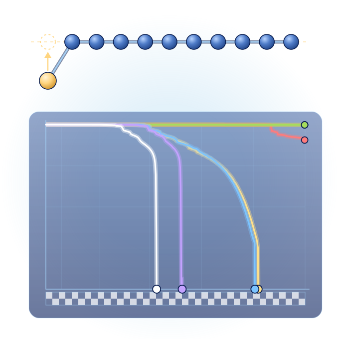
The minimiser race: eleven variables in a chain
In Part 1 the energy depended on two numbers and the walk downhill could be drawn on a map. The code written for the Training School uses eleven, linked in a chain: each variable is tied to the one before it. No map can show eleven dimensions, so here the seven methods race instead. You watch the energy of each one fall, step by step, and see how quickly the problem gets harder as the chain grows.
Based on the C++ code written by Philipp Rybakov for the POLYTOPO Training School, Budapest 2025 (acknowledgement).
Standings
The chain
The valley floor
How the difficulty grows
The race and the code
The energy of the code, for n variables x0 … xn−1. F and the variables are pure numbers without units.
F = ¼ (x0 − 1)² + Σ (xi − 2xi−1γ + 1)²
Every run starts at x0 = −1 with all other variables at 1, as in the code. The only minimum is F = 0 with all variables equal to 1. Gradient descent starts with α = 0.1 and halves it whenever a step would raise the energy.
The code is set up for n = 11 and γ = 1, with Polak–Ribière–Polyak selected, and allows up to 60 million steps. This page lets you choose n and γ and cuts every run off after 3,000,000 steps.
A run stops by itself when two steps in a row move the point by less than 10−15. The step counts leave out these last two steps. It counts as arrived if it stops closer than 0.0001 to the minimum. The methods take their steps in turn, so the race compares numbers of steps, not computing time.
Everything is computed in your browser, in double precision, with the formulas of the C++ code. The last steps depend on rounding errors, so a compiled run can differ by a few steps. If a method produces numbers that are not finite, for example when the Hessian cannot be inverted, it is marked as failed.
“Quasi-Newton” is the option named Broyden–Fletcher–Goldfarb–Shanno in the code. Its update formula is not the textbook formula of that name, so the general name is used here. With more than two variables it gives a different walk from the textbook formula.
How to use
- Press Start race. All seven methods leave the same point and take their steps in turn.
- Choose the number of variables n and the valley shape γ, and race again.
- Click a method to follow it: its chain of variables is shown on the right.
- When the race is over or paused, move Steps shown to replay it.
Reading the pictures
Race plot: one curve per method, against the step number. Both axes are logarithmic. A curve that reaches the bottom has arrived.
The chain: the variables of the followed method. All of them must reach 1. The open circles show where the valley floor lies for the current x0.
Standings: ✓ arrived, ✗ stopped short of the minimum, … cut off.
Why the race gets so hard
Each term of the energy ties one variable to the one before it. For γ = 2 the link is xi = 2xi−1² − 1. While x0 goes from −1 to 1, x1 goes down to −1 and back, x2 does so twice, and x3 four times. The number of turns of the valley floor roughly doubles with every link: 1, 3, 7, 15 and so on.
For γ = 2 the start lies on that floor, and only x0 is in the wrong place. But x0 cannot move alone: halfway along the straight line to the minimum the energy is 4.25, more than four times its starting value of 1. The methods have to find their way through the folds of the valley instead. For Newton–Raphson, each added variable multiplies the number of steps by about 2.5 to 2.7. For γ = 1 and 3 the start does not lie on the floor, and its energy is 17.
The race counts steps, not time. A step of Newton–Raphson costs far more than a step of conjugate gradient, because it fills a table of n × n numbers and solves n linear equations.
Test functions like this one are used to compare minimisers before they are applied to a real problem, such as the energy of a magnet (see Part 3). For γ = 2 it is a known benchmark of optimisation, Nesterov’s smooth Chebyshev–Rosenbrock function, with its usual starting point.
The formulas behind the picture
Energy: F(x0, …, xn−1) = ¼ (x0 − 1)² + Σi=1…n−1 (xi − 2xi−1γ + 1)². The methods are those of Part 1.
Valley floor: all terms of the sum vanish when xi = 2xi−1γ − 1 for every i. On the floor only F = ¼ (x0 − 1)² is left.
For γ = 2 the floor is xi = Tm(x0) with m = 2i, where Tm is the Chebyshev polynomial Tm(cos θ) = cos mθ. It turns m − 1 times between x0 = −1 and 1: 1,023 times for the last of eleven variables.
Sensitivity: at the minimum ∂xi / ∂xi−1 = 2γ along the floor, so a small error in x0 is multiplied by (2γ)n−1 at the end of the chain.
The C++ program written by Philipp Rybakov (University of Uppsala, Sweden) for the practical session “Numerical energy minimization in magnetics” of the POLYTOPO Training School on Physics and Mathematics of Topological Textures, Budapest, 12–13 May 2025. The test energy and the implementation of all seven minimisation methods are taken from it. The original source code is available for download and is used here with the author’s permission.
Yorgis Androulakis, IACM / FORTH
Have a suggestion to improve this simulation?